Keras learning Rate Finder
Automatically find optimal initial learning rate. See references.


- 1. Automatical learning rate finder
- 2. Initialize NN of learning rate using obtained lower-upper bounds
- References
1. Automatical learning rate finder
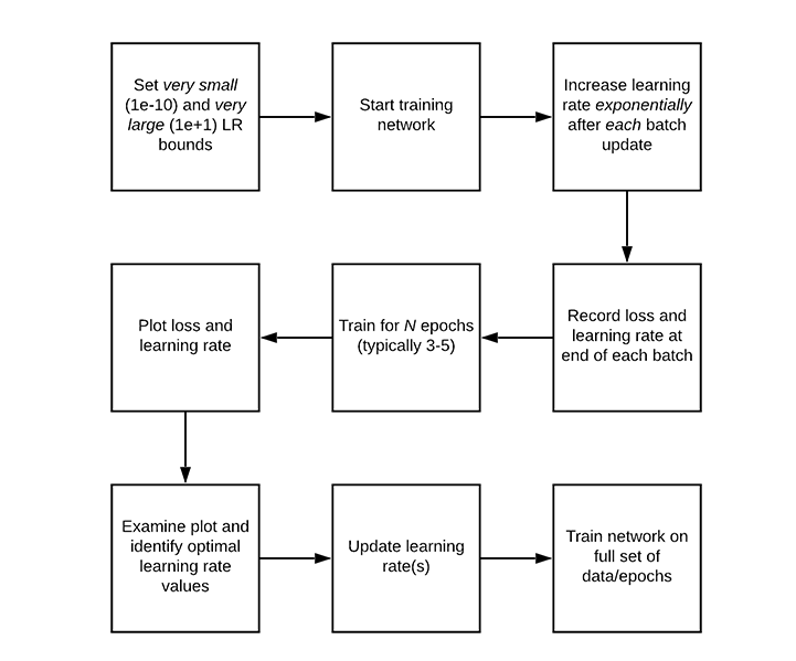
Step 1: We start by defining an upper and lower bound on our learning rate. The lower bound should be very small (1e-10) and the upper bound should be very large (1e+1).
- convergence (low lr) - divergence (high lr)
Step 2: We then start training our network, starting at the lower bound.
- after each batch we increase the learning rate --> exponentially increase
- after each batch register/save learning rate and loss for each batch
Step 3: Training continues, and therefore the learning rate continues to increase until we hit our maximum learning rate value.
- typically, this entire training process/learning rate increase only takes 1-5 epochs
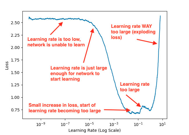
Step 4: After training is complete we plot a smoothed loss over time, enabling us to see when the learning rate is both.
-
Just large enough for loss to decrease
-
And too large, to the point where loss starts to increase
import tensorflow as tf
import matplotlib.pyplot as plt
import numpy as np
import pandas as pd
import keras
K = keras.backend
from sklearn.datasets import load_breast_cancer
from sklearn.preprocessing import StandardScaler
data = load_breast_cancer()
X_train, y_train = data.data, data.target
scaler = StandardScaler()
X_train = scaler.fit_transform(X_train)
input_  = tf.keras.layers.Input(shape = (X_train.shape[1],))
hidden1 = tf.keras.layers.Dense(units = 10, activation = "relu")(input_)
hidden2 = tf.keras.layers.Dense(units = 10, activation = "relu")(hidden1)
output  = tf.keras.layers.Dense(units = 2, activation = "sigmoid")(hidden2)
model   = tf.keras.Model(inputs = [input_], outputs = [output])

optimizer = tf.keras.optimizers.SGD()
model.compile(loss = tf.keras.losses.MeanSquaredError(), optimizer = optimizer)
class showLR(keras.callbacks.Callback) :
    def on_batch_begin(self, batch, logs=None):
        lr = float(K.get_value(self.model.optimizer.lr))
        print (" batch={:02d}, lr={:.5f}".format( batch, lr ))
        return lr

class ExponentialLearningRate(keras.callbacks.Callback):
    def __init__(self, factor):
        self.factor = factor
        self.rates = []
        self.losses = []
    def on_batch_end(self, batch, logs):
        self.rates.append(K.get_value(self.model.optimizer.lr))
        self.losses.append(logs["loss"])
        K.set_value(self.model.optimizer.lr, self.model.optimizer.lr * self.factor)
def learning_rate_finder(model, X_train, y_train, epochs, batch_size, min_rate, max_rate):
    # get weights that were used to initialize model
    init_weights = model.get_weights()
    # get and save initial leraning rate of model
    init_lr = K.get_value(model.optimizer.lr)
    # iterations = steps_per_epoch
    iterations =  epochs * len(X_train)/(batch_size) # steps_per_epoch
    # factor for computing expoenetial growth
    factor = np.exp(np.log(max_rate / min_rate) / iterations)
    # at batch = 0 set the learning rate at min_rate
    K.set_value(model.optimizer.lr, min_rate)
    # at each computed batch = 1,2,3, ... increase the learning rate by exponential growth
    exp_lr = ExponentialLearningRate(factor)
    # fit model
    history = model.fit(X_train, y_train, epochs=1, batch_size = batch_size, callbacks=[exp_lr, showLR()])
    return exp_lr.rates, exp_lr.losses

rates, losses = learning_rate_finder(model, X_train, y_train, epochs=1, batch_size=12, min_rate=0.05, max_rate = 100)
def plot_lr_vs_loss(rates, losses):
    plt.plot(rates, losses)
    plt.gca().set_xscale('log')
    plt.hlines(min(losses), min(rates), max(rates))
    plt.axis([min(rates), max(rates), min(losses), max(losses)])
    plt.xlabel("Learning rate")
    plt.ylabel("Loss")
    plt.show()
plot_lr_vs_loss(rates, losses)

References
Adrian Rosebrock, OpenCV Face Recognition, PyImageSearch, https://www.pyimagesearch.com/, accessed on 3, January, 2021> https://www.pyimagesearch.com/2019/08/05/keras-learning-rate-finder/